Analyzing DHS Data

It is important that analysts be familiar with certain key aspects of DHS data to be able to calculate accurately the indicators described in further chapters. The following sections describe some of the key elements to pay attention to in analyzing DHS data.

Sample Design, Stratification and Sampling Weights

DHS sample designs are usually two-stage probability samples drawn from an existing sample frame, generally the most recent census frame. A probability sample is defined as one in which the units are selected randomly with known and nonzero probabilities. A sampling frame is a complete list of all sampling units that entirely covers the target population.

Stratification is the process by which the sampling frame is divided into subgroups or strata that are as homogeneous as possible using certain criteria. Within each stratum, the sample is designed and selected independently. The principal objective of stratification is to reduce sampling errors. In a stratified sample, the sampling errors depend on the population variance existing within the strata but not between the strata. Typically, DHS samples are stratified by geographic region and by urban/rural areas within each region.

Within each stratum, the sample design specifies an allocation of households to be selected. Most DHS surveys use a fixed take of households per cluster of about 25-30 households, determining the number of clusters to be selected. In the first stage of selection, the primary sampling units (PSUs) are selected with probability proportional to size (PPS) within each stratum. The PSUs are typically census enumeration areas (EAS). The PSU forms the survey cluster. In the second stage, a complete household listing is conducted in each of the selected clusters. Following the listing of the households a fixed number of households is selected by equal probability systematic sampling in the selected cluster.

The overall selection probability for each household in the sample is the probability of selecting the cluster multiplied by the probability of selecting the household within the cluster. The overall probability of selection of a household will differ from cluster to cluster. See Appendix A of the DHS Survey Reports for most surveys for the details specific to that survey.

DHS dataset users should be aware that, in most cases, the data must be weighted. This is because the overall probability of selection of each household is not a constant. The following describes how DHS weights are constructed and when they should be used.

Sampling weights

Sampling weights are adjustment factors applied to each case in tabulations to adjust for differences in probability of selection and interview between cases in a sample, due to either design or happenstance. In DHS surveys, in most surveys the sample is selected with unequal probability to expand the number of cases available (and hence reduce sample variability) for certain areas or subgroups for which statistics are needed. In this case, weights need to be applied when tabulations are made of statistics to produce the proper representation. When weights are calculated because of sample design, corrections for differential response rates are also made.

There are four main sampling weights in DHS surveys: household weights, household weights for the men’s subsample, individual weights for women, and individual weights for men:

·         The household weight (hv005) for a particular household is the inverse of its household selection probability multiplied by the inverse of the household response rate in the stratum.

·         The household weight for the men’s subsample (hv028) for a particular household is the inverse of its household selection probability for the subsample multiplied by the inverse of the household response rate for the subsample in the stratum.

·         The individual weight for women (v005) is the household weight (hv005) multiplied by the inverse of the individual response rate for women in the stratum.

·         The individual weight for men (mv005) is the household weight for the men’s subsample (hv028) multiplied by the inverse of the individual response rate for men in the stratum.

There may be additional sampling weights for sample subsets, such as anthropometry, biomarkers, HIV testing, etc. There is only a need for the additional sample weights if there is a differential probability in selecting the subsamples. For example, if one in five households is selected in the whole sample for doing biomarkers, then an additional sample weight is not necessary. However, if one in five households in urban areas and one in two households in rural areas are selected, then an additional sample weight is necessary when estimating national levels or for any group that includes cases from both urban and rural areas. Notwithstanding the foregoing, the DHS has customarily included both household weights and individual weights for the subsample for the men’s surveys, normalizing the weights for the number of households in the subset for the men’s surveys, and to the number of men’s individual interviews even when no differential sub-selection has been used.

Response rate groups are groups of cases for which response rates are calculated. In DHS surveys, households and individuals are grouped into sample strata and response rates are calculated for each stratum.

Household Response Rate

Coverage: All households. Excluded are dwellings without a household (no household lives in the dwelling, address is not a dwelling, or the dwelling is destroyed).

Numerator: Number of households with a completed household interview (hv015 = 1).

Denominator: Number of households with a completed household interview, households that live in the dwelling, but no competent respondent was at home, households with permanently postponed or refused interviews, and households for which the dwelling was not found (hv015 in 1, 2, 4, 5, 8).

The household response rate for the men’s subsample is calculated in the same way but restricting numerator and denominator to household selected for the men’s subsample.

Women’s Individual Response Rate

Coverage: Women eligible for interview, usually women age 15-49 who stayed in the household the night before the survey. In ever-married samples, women are eligible for interview only if they have ever been married or lived in a consensual union. In some surveys, the age range of eligibility has differed, e.g., ever-married women age 12-49.

Numerator: Number of eligible women with a completed individual interview (v015 = 1).

Denominator: Number of eligible women with a completed individual interview, eligible women not interviewed because they were not at home, eligible women with permanently postponed or refused interviews, eligible women with partially completed interviews, eligible women for whom an interview could not be completed due to incapacitation or other reasons (v015 in 1:9).

Men’s Individual Response Rates

Coverage: Men eligible for interview, usually men age 15-49, 15-54, or 15-59 who stayed in the household the night before the survey. In ever-married samples, men are eligible for interview only if they have ever been married or lived in a consensual union. The age range of eligibility varies from survey to survey.

Numerator: Number of eligible men with a completed individual interview (mv015 = 1).

Denominator: Number of eligible men with a completed individual interview, eligible men not interviewed because they were not at home, eligible men with permanently postponed or refused interviews, eligible men with partially completed interviews, eligible men for whom an interview could not be completed due to incapacitation or other reasons (mv015 in 1:9).

Normalization of Weights

Sample design weights are produced by the DHS sampler using the sample selection probabilities of each household and the response rates for households and for individuals. The initial design weights are then normalized by dividing each weight by the average of the initial weights (equal to the sum of the initial weight divided by the sum of the number of cases) so that the sum of the normalized weights equals the sum of the cases over the entire sample. The normalization is done separately for each weight.

Application of Sampling Weights

Sample weights are calculated to six decimals but are presented in the standard recode files without the decimal point. They need to be divided by 1,000,000 before use to approximate the number of cases. Sampling weights can be applied in two main ways:

1)      A simple application of weights when all that is needed are indicator estimates.

2)      As part of complex sample parameters when standard errors, confidence intervals or significance testing is required for the indicator.

The methods of applying the weights varies across the various statistical software.

Example 1: Simple weighting

The below examples for Stata, SPSS and R produce simple weighted estimates of current use of modern methods. Note that any standard error or confidence interval given by the below commands assume a simple random sample and do not take into account the complex sample used in DHS surveys.

Complex sample designs

However when standard errors, confidence intervals or significance testing is required, then it is important to take into account the complex sample design. For the complex sample design, it is necessary to know three pieces of information – the primary sampling unit or cluster variable, the stratification variable, and the weight variable.

The primary sampling unit variable is typically v021 (or hv021 or mv021). If this variable does not contain the PSU number, then, in all but a few surveys, the cluster number (v001 or hv001 or mv001) can be used. In most surveys there is a one-to-one correspondence between the cluster number and the PSU number, but in a small number of surveys, for example some of the surveys in Egypt, the PSU and cluster number do not match one-to-one – see Appendix A in the DHS survey reports for details of the sampling design.

The stratification variable is typically v023 (or hv023 or mv023), however the stratification variables have not been consistently defined in many surveys and may need to be created. It is best to check the sample design in Appendix A of the DHS survey reports to verify the stratification used in the design of the sample. In many surveys, the stratification is based on urban and rural areas in each region (v024 x v025).

The weight variable is v005 (or hv005 or mv005) divided by 1,000,000.

To apply the complex sample design parameters in estimating indicators each of the statistical software use a different set of commands applying the sample design and producing the indicator estimates:

Stata:    svyset and svy: commands

SPSS:     csplan, csdescriptives and cstabulate commands

R:            survey package, including svydesign and other svy functions.

Example 2: Complex sample design weighting

The below examples for Stata, SPSS, and R, continuing on from example 1, demonstrate the use of the complex sample designs for estimates of current use of modern methods, together with standard errors and confidence intervals.

Notes and Considerations

The sum of the sample weights only equals the number of cases for the entire sample and not for subgroups such as urban and rural areas.

Sample weights are inversely proportional to the probability of selection and are used to correct for the under- or over-sampling of different strata during sample selection. If weights are not used, all calculations will be biased toward the levels and relationships in the over-sampled strata. Comparisons of regression coefficients, as well as rates, percentage, means, etc. coming from different surveys are only valid if weights have been used to correct for the sample designs of the different surveys.

An option to use sample weights is included in virtually all procedures in all statistical packages. Weights tend to increase the size of standard errors and confidence intervals, but not by large amounts. Recommendations against the use of weights for estimating relationships, such as regression and correlation coefficients, in prior versions of the Guide to DHS statistics are no longer DHS policy.

For more information on DHS sample design, stratification and sample weights, see the DHS Sampling and Household Listing Manual (https://www.dhsprogram.com/publications/publication-DHSM4-DHS-Questionnaires-and-Manuals.cfm). See also the DHS YouTube videos:

Part I: Introduction to DHS Sampling Procedures

Part II: Introduction to Principles of DHS Sampling Weights

Part III: Demonstration of How to Weight DHS Data in Stata

Part IV: Demonstration of How to Weight DHS Data in SPSS and SAS

Setting the survey design using DHS data in R - Part 3

Households

Households are the primary unit selected for interview in DHS surveys. The definition of a household is a person or group of related or unrelated persons who live together in the same dwelling unit(s), who acknowledge one adult male or female as the head of the household, who share the same housekeeping arrangements and who are considered a single unit.

Each country has its own definition of a household, which may vary slightly from this definition, but generally the definition is very similar.

De Facto and De Jure Populations

When listing household members in the roster of a DHS Household Questionnaire, the household respondent is asked “Please give me the names of the persons who usually live in your household and guests of the household who stayed here last night, starting with the head of the household.” For each person listed the respondent is asked “Does (NAME) usually live here?” and “Did (NAME) stay here last night?” For most people listed, the answer to both questions will be yes. However, there are some people for whom the respondent says yes, they usually live in the household, but no, they did not stay in the household the previous night. Conversely, there may be some guests who do not usually live in the household but stayed in the household the previous night.

The group of people that usually live in the surveyed households are known as the de jure population (or usual residents) and the group of people that stayed in the household the previous night are known as the de facto population. Typically, more than 90 percent of the persons listed in the household roster are both de jure and de facto household members.

Theoretically a person could be a de jure member in one household and a de facto member in another household and could potentially be included more than once in the survey. To avoid this potential double counting of people it is important to ensure that either a de facto population or a de jure population is selected for all analysis of the data. Either one is a valid population. DHS generally selects a de facto sample as the response rate is usually higher for the de facto population as they stayed in the household the previous night and are less likely to be away. The DHS individual women’s recode (IR file) and men’s recode (MR file) only contain de facto women and men respectively.

In the household members recode (PR file), all persons listed in the household roster are included in the file and the choice of population for reporting may differ depending on the indicator. For example, for anthropometric measures, anemia testing, and HIV testing, The DHS Program selects the de facto population as the persons must be measured and tested and the response rate is typically higher for this group. However, for indicators that are about the household, such as the water and sanitation indicators, and where the person may not be interviewed themselves, The DHS Program reports based on the de jure population as the person usually lives in the household and uses the water and sanitation facilities, whereas the water and sanitation facilities used by any guest in the household may be quite different in their own household compared to the surveyed household.

For all indicators based on the household members (PR file), either the de jure population (hv102 = 1) or the de facto population (hv103 = 1) is selected. See the YouTube video on De Jure and De Facto for more information.

Age of Children

The age of children is used frequently in selecting the children to be included in the denominators and numerators of many of the indicators described in the following chapters. In DHS-7, The DHS Program changed the way in which the age of children is calculated to provide a more accurate estimate of their age. Day of birth was added for all births in the birth history in DHS-7 questionnaires. Adding day of birth permits the calculation of ages of children in days, and allows for the more accurate calculation of age in months (https://www.dhsprogram.com/data/calculating-the-age-of-children.cfm).

Due to the addition of the age in days, The DHS Program also introduced the Century Day Code (CDC) – the number of days since January 1, 1900. Several variables related to the century day codes have been added, and as well as several new age-related variables:

v008a:                   CDC date of individual interview, similar to the century month code variable v008.

b17:                       Imputed day of birth for children of the respondent (similar to the imputed month and year of birth in b1 and b2).

b18:                       CDC date of birth of children of the respondent.

b19:                       Age of child, or months since birth for children who have died, in completed months, computed as:

                                b19 = int( (v008a - b18) / 30.4375)

hv008a:                CDC date of household interview

hv807a:                CDC date of biomarker data collection

hml16a:                Age of child in months for children. Used for reporting malaria testing for children

hc1a:                     Age of child in days for children included in the biomarker questionnaire

hc20:                     CDC date of biomarker data collection for children. If date of measurement is included for individual children the variable may be different than hv807a, for example when retaking child’s measurements

hc32a:                   CDC date of birth of children included in the biomarker questionnaire

hw1a:                    Age of child in days for children included for anthropometry in the biomarker questionnaire

Changes have also been made to the method of calculating several existing variables:

b8:                          Age of child in years – now calculated based on b19, instead of v008 - b3

b11, b12:             Previous and succeeding birth interval. Previous birth interval was previously calculated as b3(i) - b3(i+1), but is now calculated as int( (b18(i) - b18(i+1)) / 30.4375 ), and a similar change is made for the succeeding birth interval

v208:                     Births in the five years preceding the survey

v209:                     Births in the 12 months preceding the survey

v222:                     Interval between last birth and date of interview in months

v238:                     Births in the three years preceding the survey

v337:                     Months of use of current contraceptive method

hc1:                        Age of child in months for children for whom anthropometric measures were taken, computed as follows:

                                hc1 = int( (hv807a - hc32a) / 30.4375 )

hw1:                      Age of child in months for children of respondents for whom anthropometric measures were taken. hw1 is set equal to hc1. Take note that hc1 and hw1 are calculated with reference to the date of biomarker data collection, and this can occasionally differ from the date of individual interview, and so, on rare occasions hw1 and b19 may differ slightly.

hml16:                  Age of child in months for children included in the malaria bed net roster

Additionally, anywhere that a restriction based on the age of the child or the number of months since a birth, e.g. selecting all children born in the last five years, the condition has been changed to refer to b19 instead of v008 - b3.

In surveys that introduced the day of birth of the child, changes have been made in the analysis of the data in two main ways:

1)      The restrictions on the denominator for tables now all use the age variables based on the calculation to the day, rather than to the month. In most cases this means changing selections such as

if (v008 - b3 < 60)

                to

                                if (b19 < 60)

If the original restriction is applied, the analysis will exclude a small number of cases that are included with the newer calculation. On average, this will add approximately half a month’s worth of additional births or children into the analysis.

2)      All background age group variables used in analysis are now based on the revised ages. Previously on average, because the calculation method only considered month and year and not day of birth, the age group of 0 months would have roughly half the number of cases of age group 1 month, or other older single month age groups. With the new method, age group 0 months will have a roughly similar number of cases as other single month age groups.

These changes affect virtually all tables related to children, particularly to children under the age of five.

Fertility rate and childhood mortality rate tables are not currently changed as these tables exclude the month of interview from calculations and effectively use complete months in the calculations.

For analysts it is recommended that they change their selection criteria in analysis from using v008 - b3 < xx to b19 < xx. It is possible to generalize the logic changes to creating b19 using the old approach if it does not exist in the dataset, or to use b19 if it does exist. Below are examples for use in Stata and SPSS:

This approach will use b19 if it exists in the dataset, but otherwise create its equivalent using the old age calculation method and allow the production of analyses that are consistent with the tabulations in the DHS reports.

All Women Factors

Definition

Factors for adjusting ever-married samples to estimate statistics based on all women.

Coverage:

Population base: All de facto women (PR file)

Time period: Current status at time of survey

All women factors are specific for individual years of age and specific for the particular subgroup to be estimated (e.g., there are two sets of factors by type of area: one for urban areas and one for rural areas).

Numerator: Number of all de facto women age 15-49 (hv103 = 1 & hv104 = 2 & hv105 in 15:49), by single years of age (hv105) and background characteristics

Denominator: Number of de facto ever-married women age 15-49 (hv103 = 1 & hv104 = 2 & hv105 in 15:49 & hv115 in 1:9), by single years of age (hv105) and background characteristics

Variables: PR file.

Calculation

Numerator: From the household survey, tabulation by single year of age and by subgroup of the number of women 15–49 years of age of any marital status who slept in the household the night before the interview.

Denominator: From the household survey, tabulation by single year of age and by subgroup of the number of women age 15–49 years who slept in the household the night before the interview who have ever been married.

Tabulations use the household sampling weights (hv005).

All women factors are numerator divided by denominator. Factors are multiplied by 100 in the recode file.

Example:

The following table shows an example of the number of women age 15-49 for all women, ever-married women and the resulting all women factors according to place of residence(urban/rural) and total. The distribution was obtained from the household schedule for de facto women (women who stayed in the household the night before the survey). The data are weighted using the household weights.

The “all women factors” are calculated by dividing the total number of women by the number of ever-married women for each characteristic (urban/rural and total )within each single age. The factor for women 15 years old living in rural areas is 9.5 or an ever-married woman age 15 living in a rural area represents 9.5 women of the total women population in that area for that survey. This value is calculated by dividing 413.65 by 43.55.

It is important to note that there are no ever-married women for ages 15 and 16 in the urban areas. To calculate the factors for those ages, the total number of women needs to be accumulated until an age where ever-married women are found (age 17 in this case). The result of this accumulation is then divided by the number ever-married women found.

(50.70 + 48.18 + 41.07)/15.84 = 139.95/15.84 = 8.84

The same factor is applied to women ages 15, 16, and 17 because 15.84 ever-married women represent the 139.95 accumulated women for those age groups.

Handling of Missing Values

Women with missing or unknown age are excluded from both the numerator and the denominator. Women with unknown or missing marital status are considered never-married.

Notes and Considerations

Women in consensual unions and women separated from consensual unions are considered as ever- married.

If there are no or very few women ever-married for a single age for the subgroup, then neighboring ages are combined to calculate the all women factor, using the same value for each of the single ages.

The all women factors for ever-married samples are the inverse of the proportions ever-married at the time of the survey.

The all women factors are used because of the selection process used in the design of the sample. Therefore, it is only appropriate to use internally generated factors and not to use information external to the survey. For each subgroup to be estimated, the same factor is applied to each woman irrespective of the time period to be estimated since it is based on sample selection.

In surveys using samples of ever-married women and ever-married men, the same methodology is used to calculate all men factors.

Although the factors are calculated at the household level, they are normally used at the women’s level (or men’s levels for ever-married men’s surveys). To do that, each woman is assigned a factor for each characteristic for which the factors are calculated.The links to assign the factors are age and the characteristic. In the example above an ever-married woman 18 years old, living in an urban area, would be assigned the factors 1.32 for the total (awfactt = 132) and 2.11 for place of residence (awfactu = 211). When establishing the values for the characteristics to be used as links, they must be taken from the household members data (PR file) and not from the woman’s data. The reason is that there may be differences from the data reported in theHousehold Questionnaire compared with the data recorded in the Woman’s Questionnaire. A different person than the respondent to theWoman’s Questionnaire may report age and education of the woman in theHousehold Questionnaire. However, when factors are calculated they need to use the household variables (because not all women have an individual interview).

Another important issue is that factors can only be calculated for characteristics present in the Household Questionnaire. For example, factors for media exposure or knowledge of HIV/AIDScannot be calculated because they are collected at the women’s level.

The appropriate all women factor to use in analysis is that of the woman’s reported single year of age from the household survey at the time of the survey for the subgroup to be tabulated. Fortunately the DHS individual recode files already includes the all women factors. DHS individual woman’s recode files (IR files) include five standard variables containing all women factors:

·         awfactt         All women factor for total population

·         awfactu        All women factor for place of residence (urban/rural)

·         awfactr         All women factor for region (according to the country’s regions)

·         awfacte        All women factor for education (none, primary, secondary, higher)

·         awfactw       All women factor for wealth index (lowest, second, middle, fourth, highest)

Surveys may also include additional all women factors for other background characteristics, particularly when survey specific educational groupings are used.

These variables are five-digit variables with two implicit decimals, so they must be divided by 100 before applying. Any table that is based on total population for ever-married samples should use these factors. All tables based on all women (fertility rates, age at first union, age at first sex, etc.) must use all women factors. If the background variable to be used is not one of the standard or country-specific all women factors they have to be created as described above.

The “all women” factor is sometimes known as the “all woman” factor and variables may be named either way in the data files.

Application of All Women Factors

In tabulations, all women factors are treated as adjustments to the respondent sampling weight variable for each woman, multiplying the weight variable for the woman by her appropriate all women factor to inflate the number of cases from the number of ever-married women to the number of all women. In many cases though it is not as simple as multiplying the sampling weight by the all women factor. For example, to calculate the percentage married before age 15 of all women from an ever-married sample, simply applying the all women factor to the weight variable would be to assume that the same proportion of never-married women were married before age 15 as ever-married women, and this is clearly impossible. Rather we know that no never-married women aged 15 and older were married before age 15. In terms of the calculation, this means that the all women factor must be applied to the denominator only, and not to the numerator.

Similarly, to calculate the mean number of children ever born for all women from an ever-married sample, the assumption is made that never married women have had no children. Thus it is not necessary to increase the numerator (the number of children ever born) as there are no children to add, but it is necessary to inflate the denominator to include all women.

In practice, using statistical software, it is typically not possible to use simple percentages or means when using all women factors, but rather to calculate ratios of variables. Below are examples of calculating the mean number of children ever born in Stata and SPSS:

Note that in SPSS the ratio statistics command does not permit non-integer weights so v005 is used as the weight directly without dividing by 1,000,000.

Median Calculations

There are four different types of median calculations in DHS statistics, and results vary according to the type of variable being analyzed. The calculations for the first three types of medians are calculated in a similar manner and vary basically in the final result. Medians using the current status data are calculated using a different methodology. To illustrate the approach used in calculating the first three types of medians, consider the following table, which will be used in examples below:

Medians for Completed Time Periods

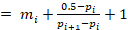
These are medians for variables such as intervals between events or ages calculated at different events. Medians for this type of variable take into consideration that ages are given in completed years. The median for completed time periods is calculated as:

median  

where i is the age category immediately prior to reaching 50%, mi is the number of completed years for that category, p i is the cumulative proportion at the age category immediately prior to reaching 50%, and p i+1 is the cumulative proportion at the age category immediately after reaching 50%.

A respondent who is currently 21 years old could be somewhere between 23 years and 0 days old and 23 years and 364 days old. The addition of 1 in the calculation is because the cumulative percentage for a particular category is the percentage up to the end of the category. For example, the cumulative percentage for age 23 is the cumulative percentage by age 24.

Example

If the variable above in question is age at an event in completed years, the median would be calculated for a completed period. In this case the interpolation will take place between the ages of 23 and 24. The result of the interpolation is 23 + (50 - 43)/(52 - 43) + 1 = 24.8. The one year has to be added as, according to the completed year definition of age, the cumulative percentage of 43 percent occurred before reaching 24 years and the cumulative value of 52 percent occurred before reaching 25 years of age.

Examples of these types of medians are age at first sexual intercourse, age at first union, age at first birth, age at sterilization, median number of months since preceding birth, and median number of months pregnant at time of first antenatal care visit.

Medians for Continuous Variables

These are medians for variables such as children’s weight at birth or any other type of measurement in the continuous scale. The median for continuous variables is calculated as:

median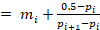  

where i is the entry immediately prior to reaching 50%, mi is the value for that entry, p i is the cumulative proportion at the value immediately prior to reaching 50%, and pi+1 is the cumulative proportion at the value immediately after reaching 50%.

Example

If the variable in the table above was continuous, for example, time to collect water (for purposes of simplicity, time is truncated to the minute). The interpolation would also take place between 23 and 24 minutes, and no adjustment is needed. The median time to collect water would then be 23.8 minutes.

The standard DHS-7 tabulation plan currently includes no examples of medians for continuous variables, although median time to collect water, or median birth weight are examples of this type of median that could be calculated using DHS data.

Medians for Discrete Variables

These types of medians apply to variables such as number of children, number of antenatal care visits, or in general any discrete variable where the only possible values are integers. For example, a respondent can only have one, two, or any integer number of children. It is not possible to have 2.3 children.

If the variable is discrete, the median would be obtained at 24 when 50 percent or more was reached. However, it is also possible to present an interpolated median for discrete variables, and in this case the same formula is used as for continuous variables. Examples of these medians in the Guide to DHS Statistics include median years of education in Chapters 2 and 3.

Medians using Current Status Data

These types of medians are calculated for variables where 100 or close to 100 percent of the population have a characteristic at the beginning of an event and the percentages diminish as time passes by. For example, 100 percent of children do not know how to walk at birth. As time progresses, some children begin to walk, and there is an age (in months) where 50 percent or more of the children learn to walk.

Current status data are used in DHS to calculate the median duration of breastfeeding, post-partum amenorrhea, post-partum abstinence, and post-partum insusceptibility. Looking at how the median duration of breastfeeding is calculated(the same principle applies for amenorrhea, abstinence, and insusceptibility), information is first obtained on the proportion of children currently being breastfed (for breastfeeding, according to the children’s age in months).For purposes of providing some stability to the proportions, the birth data are grouped into two-month intervals. Before calculating the proportions, the distribution is smoothed by a moving average of three groups.

To smooth the distribution by a three-group moving average, sum the previous, current, and following value of the distribution and divide it by 3. For example, the smoothed total children for the age group 2–3 comes from: (137.6 + 183.0 + 193.4)/3 = 171.3. The first (0–1) and last (34–35) age groups cannot be smoothed, so they remain with the original values. The number of children currently being breastfed is also shown unsmoothed and smoothed. With the distributions smoothed, the percentages of children in each group are calculated:

The first age (duration) for which the proportion falls below 50 percent will be used for the calculation of the median by linear interpolation between the midpoint of that age group and the next youngest midpoint age. The median in this example falls between the age groups 18–19 and 20–21. Between these two age groups is when the transition from more than 50 percent (51.9%) to less than 50 percent (43.1%) of children still being breastfed occurred. The interpolation is then done between the midpoints for the age groups. In DHS-7, the midpoint of the 18-19 month age group is the average of the lower and upper limits of the age group (18.0+20.0)/2 = 19.0. Similarly for age group 20-21 the midpoint is 21.0. Note that in DHS-VI and earlier phases the midpoints would have been 18.5 and 20.5 respectively due to the different calculation of age (the age distribution would also be different though). This is because, prior to DHS-7, the age of children was calculated in months only, and the month of interview was on average only half a month, and consequently all following month groups had a midpoint half a month less.

It should be noted that, in DHS-VI and earlier, the midpoint for the first age group is calculated in a somewhat different manner. On average, there were only about half as many children born in the month of the interview than in any other regular month. A reasonable age for children born in the month of interview was 0.25, assuming that interviews are uniformly distributed. Thus, the age average for kids born 0 to 1 months was calculated as (0.5 * 0.25 + 1)/1.5 = 0.75. In DHS-7, the midpoint for the first age group is simply (0.0 + 2.0)/2 = 1.0.

The median is calculated using the following formula:

median = mi + (mi+1 - mi) . (p i - 0.5) / (p i - p i+1)

median = 19.0 + (21.0 – 19.0) . (51.9 – 50.0) / (51.9 – 43.1)

median = 19.4

Details of the calculation of these medians are provided with each indicator in the chapters that follow.

Matching and Merging Datasets

The DHS Program distributes separate datasets for households (HR), household members (PR), women’s (IR), births (BR), children under five (KR), men’s (MR), and couples(CR) files. Care has been taken to include all variables deemed important for each of these files.For example, variables for household characteristics are included in the women, men, and children’s files. However,there are instances when researchers need to merge or combine different files to obtain the variables that meet their analysis requirements. This section discusses the variables and mechanisms that can be used to accomplish that task.

ID Variables

One of the advantages of processing complex surveys with a software capable of handling hierarchical files is that it allows tight control of the case identifiers. The DHSProgram makes considerable effort to ensure that files can be matched seamlessly whenever a relationship is possible. To properly manipulate the files it is necessary to know the variables that identify cases in each file. The following table shows those variables:

The ID variables hhid, caseid, and mcaseid are alphabetic variables that uniquely identify households, women, and men respectively. These variables are a concatenation of the cluster number and household number for the household file, and cluster, household number, and line number for women, men, and couples. The variable hhid is a 12-character string with the cluster and household number right-aligned in the string. The variables caseid and mcaseid are 15-character strings with the cluster, household, and line number right-aligned in the string. The first 12 characters of variables caseid and mcaseid match with hhid and are followed by 3 characters for the line number. In the concatenated variables numbers are converted to strings with leading blanks for each part of the ID.

Example

Note: A dot (.) is used above to represent a blank in the ID values.

The layout of the hhid and caseid strings will vary depending on the number of digits used for the cluster and household number in the survey. In addition, some surveys also include a dwelling number in the hhid and caseid string between the cluster and household number.

In the case of children, variable caseid is the same as that of their mother plus a consecutive number to differentiate among children in reverse chronological order. The ID for couples is that of the woman (caseid - as opposed to mcaseid for the man) because in polygynous countries a man can be the partner for more than one woman.

Type of Relationship

When merging data files it is important to know the type of relationship that exists between the files to be merged as well as the type of output file desired (unit of analysis). There are two main types of relationships: The first is that of many entities related to one entity (m:1) and the second is that of one entity related to just one other entity (1:1). A third possibility is a many-to-many relationship, but that is not generally used in analyzing DHS data.

An example of many-to-one relationships can be found between women or men and households. There may exist zero or several Woman’s or Man’s Questionnaires for each household (see Structure of DHS Data), and there is just one household that will match each woman or man.

An example of one-to-one relationships can be found between children of interviewed women in the KR file and the children’s records as household members in the PR file. There will be at most one record in the PR file for a child in the KR file, but there could be no record in the PR file if the child has died or the child does not live in the household. [Note – however, that when merging PR data for a child to the KR data, it may be necessary to define the relationship as many-to-one (m:1) as the household line number will be not applicable (missing in Stata, system missing in SPSS) for any child who has died or lives elsewhere and is not listed in the household schedule, and these may appear as duplicate IDs.]

In some surveys, the couple’s relationship between a woman and man may be considered a one-to-one relationship, but in many surveys, there are polygynous unions and so the relationship is usually a many-to-one (m:1) relationship between women and men.

Merging Files

All statistical packages, including Stata, SPSS, SAS, and R, have commands that allow merging of files, but regardless of the software the following steps are necessary:

·         Determine the common identifiers (identification variables)

·         Determine the base (primary) file. The base file essentially establishes the unit of analysis

·         Determine the variables to merge from the secondary file to the primary file

·         Ensure both data files are sorted by the identification variables

·         Finally, use the right commands for the software to merge the files

Normally, when the relationship is that of many-to-one (m:1), the base file is the one with the many entities. For example, if merging data from households and women, the base file should be the women’s file because this will assign to every woman the characteristics of her household. If the match is done the other way around, in some software, once the program matches the first woman it will not look for another woman or it will give an error for finding duplicate cases. In the case of matching women and children, the base file should be the children’s file, and the mothers’ characteristics are assigned to children.

In DHS surveys, Man’s Questionnaires are often applied to a subsample of households. This means that not all currently married women have a match with a Man’s Questionnaire. In this case, the base file should be the Man’s Questionnaire and the resulting file (unit of analysis) will be the Couples file.

If the relationship is that of one-to-one (1:1), the base file is normally the one with the smaller number of cases.

Merging can be performed using either the ID variables (hhid, caseid, mcaseid) or using the cluster number (hv001, v001, mv001), household number (hv002, v002, mv002), and household line number (hvidx, v003, mv003, or other line number variables). Most matches will work using either set of information in most cases, but there are some issues with some surveys:

·         The ID variables are left-aligned in a few surveys, rather than right aligned, complicating converting caseid to hhid. This can be corrected by right aligning the variable:

Stata: replace hhid = substr("      ",1,12-length(hhid)) ///

       + substr(hhid,1,length(hhid))

SPSS:  compute hhid = concat(char.substr("      ",1,12-char.length(hhid)),

char.substr(hhid,1,char.length(hhid))).

·         In some surveys hhid has a different length than 12 or caseid or mcaseid has a different length than 15. These can usually be corrected to the right length, but care should be taken to ensure that no data are lost from the IDs in the process.

·         The combination of cluster, household and line number is not unique in some surveys. For these surveys, typically there is also a dwelling number which must be used, and the household number is the number within the dwelling. For these surveys it is necessary to include the dwelling number in the set of variables used for matching. The dwelling number will usually be a survey-specific variable starting with “sh”, “s”, or “sm” for household, woman’s and man’s files.

Examples

The following is a list of common combinations of datasets that may be merged together:

A few of these types of merges are not typically needed as the variables of interest are already included in the base file.

Most merges can be done in a number of ways, but typically follow the approach of:

1.       Opening the secondary file and extracting just the variables that need to be merged together with the ID variables for matching, sorting the data on the ID, and saving into a temporary file. This may include renaming ID variables or variables to be merged to facilitate the merge.

2.       Opening the primary file, ensuring that the same ID variables are available, sorting on the IDs.

3.       Merging as a many-to-one (m:1) or one-to-one (1:1) match on the ID variables.

Below are a few examples in Stata and SPSS of typical merges from the list above.

Example 1:

This example merges household characteristics from the household (HR) file to the children under five (KR) file. This is a relatively simple merge based on the household ID using either hhid or the combination of cluster number and household number. When using the household ID (hhid) it is necessary to construct this from the caseid variable in the KR file for matching. Alternatively, using the cluster number and household number, the variables in the household file are renamed to permit matching. Either approach to matching should produce the same results.

Note for SPSS users: If the string variables for hhid or caseid are three times the expected size (expected size: 12 for hhid and 15 for caseid), the file was opened in Unicode mode. Close the file, set unicode off, and retry.

Example 2:

This example merges mother’s characteristics from the household members (PR) file to the children’s records in the household members (PR) file. This example looks complicated in that both the base file and the secondary file are the same file but is relatively simple. It requires creating a simple file of the selected characteristics, with the ID variables, and then matching that file to the PR file based on the correct IDs. A person ID variable (pid) is created for use in matching and is based on the household member line number in the secondary file, and on the mother’s line number in the primary file. This will match only for the children whose mother is also listed in the household members file.

This approach can also be used to match women’s characteristics from the IR file to the children’s characteristics in the PR file. The only differences are in creating the temporary file, based on the IR file data. It requires constructing hhid from caseid as in the prior example (or using the cluster and household number) and creating pid from the woman’s line number (v003).

Example 3:

This example merges children’s characteristics from the household members (PR) file to the children under five (KR) file. In this example, rather than creating the matching variables in the secondary file, they are created in the base file. In Stata, because b16 will be missing for dead children or children living elsewhere, the merge must be treated as many-to-one (m:1), even though the cases actually merging will be one-to-one (1:1). This is because the IDs must be unique for a 1:1 match, but as more than one case within a household may be missing for b16, they are not unique. The KR file could be subset to only include children listed in the household before the merge, and then a 1:1 match can be used.

Example 4:

This example merges HIV test results from the AR file to the women’s data (IR) file. In this example, the hhid and caseid variables do not exist in the AR file, so the merge will be based on the cluster, household, and line number variables. The relationship between the cases is a 1:1 match, and the women’s data will be the base file.

Background Characteristics

In most DHS report tabulations, results are presented by background characteristics. These characteristics fall into groups according to the unit of analysis to which they apply. These units include the cluster, household, household member, individual woman respondent, individual man respondent, birth, or child. Characteristics from higher levels may also be used in tabulations at lower levels. For example, cluster level characteristics such as region and type of place of residence are used at all levels, and individual women’s characteristics such as level of education may be used when reporting on their children.

The main background characteristics are described here briefly for each of these units:

Cluster

Region of residence

Region of residence (hv024, v024, v101, mv024) is defined for every cluster or enumeration area as part of the sample design for the survey. Region of residence is typically the first administrative level within the country, or a grouping of the first administrative level.

Type of place of residence

Type of place of residence (hv025, v025, v102, mv025) is the designation of the cluster or enumeration area as an urban area or a rural area. As for region of residence, the type of place of residence is established for the cluster as part of the sample design for the survey and cannot vary within cluster.

The definition of a cluster as urban or rural is made according to the definition used in each country. The traditional distinction between urban and rural areas within a country has been based on the assumption that urban areas, no matter how they are defined, provide a different way of life and usually a higher standard of living than rural areas. In many developed countries this distinction has become blurred, and the principal difference between urban and rural areas in terms of living standards tends to be the degree of population concentration or density (UNSD, 2017). UNSD recommends that the classification of a cluster as urban or rural is made first and foremost on a measure of population density. However, other criteria may also be considered in the designation of the cluster, including the percentage of the population involved in agriculture, the availability of electricity or piped water, and the ease of access to healthcare, schools, or transportation, among others. There is no one standard definition of urban and rural, and the definition used is necessarily country specific and may change over time.

Household

Wealth Quintile

The wealth index (hv270, v190, mv190) is a composite measure of a household's cumulative living standard. The wealth index is calculated using data on a household’s ownership of selected assets. Information on the wealth index is based on data collected in the Household Questionnaire. This questionnaire includes questions concerning the household’s ownership of a number of consumer items such as a television and car; dwelling characteristics such as flooring material; type of drinking water source; toilet facilities; and other characteristics that related to wealth status.

Each household asset for which information is collected is assigned a weight or factor score generated through principal components analysis. The resulting asset scores are standardized in relation to a standard normal distribution with a mean of zero and a standard deviation of one.

Each household is assigned a standardized score for each asset, where the score differs depending on whether or not the household owned that asset. These scores are summed by household, and individuals are ranked according to the total score of the household in which they reside. The sample is then divided into population quintiles -- five groups with the same number of individuals in each to create the break points that define wealth quintiles as: Lowest, Second, Middle, Fourth, and Highest.

The asset index is developed on the basis of data from the entire country sample and used in most tabulations presented, based on separate scores prepared for rural and urban households, and combined together to produce a single asset index for all households.

Wealth quintiles are expressed in terms of quintiles of individuals in the population, rather than quintiles of individuals at risk for any one health or population indicator.

See https://www.dhsprogram.com/topics/wealth-index/Index.cfm for more information on the wealth index, and particularly:

·         DHS Comparative Reports No. 6, The DHS Wealth Index (Rutstein and Johnson, 2004) https://www.dhsprogram.com/publications/publication-cr6-comparative-reports.cfm for the original approach to the creation of the wealth index, and

·         DHS Working Papers No. 60, The DHS wealth index: Approaches for rural and urban areas (Rutstein, 2008) https://www.dhsprogram.com/publications/publication-WP60-Working-Papers.cfm for the revised approach.

Source of drinking water

The main source of drinking water (hv201) for members of the household is classified as improved and unimproved sources, following the WHO/UNICEF Joint Monitoring Programme (JMP) on Water and Sanitation guidelines. The JMP provided an updated methodology for this classification in 2018 and this was implemented in DHS surveys in September 2018 (WHO/UNICEF, 2018). Typically, this is used as a characteristic related to prevalence of diarrhea.

Type of toilet facility

The type of toilet facility (hv205) members of the household usually use is classified into groups for improved sanitation, unimproved sanitation: shared facility, unimproved sanitation: unimproved facility, and open defecation, following the WHO/UNICEF Joint Monitoring Programme (JMP) on Water and Sanitation guidelines. As for source of drinking water, the updated JMP methodology was implemented in DHS surveys in September 2018 (WHO/UNICEF, 2018). Typically, this is used as a characteristic related to prevalence of diarrhea.

Cooking fuel

The main type of cooking fuel (hv226) used by the household is used as a characteristic related to prevalence of symptoms of acute respiratory infections (ARI).

Household Member

Sex

Sex of each household member (hv104) is collected in the Household Questionnaire with the question: “Is (NAME) male or female?”. The DHS Program does not typically collect data for any other categories. Respondents are permitted to refuse to answer, and their responses will be excluded from any sex-specific results.

Age

Age of each household member (hv105) is asked in the Household Questionnaire with the question “How old is (NAME)?”. Age is recorded in completed years, with children under one year recorded as 0 years old. Ages above 95 are recorded in a category of 95 or more.

Education

Education is generally reported as the highest level of education attended (not necessarily completed) (hv106 or hv109) in categories of no education, primary, secondary, higher than secondary. The classification of education used in the tabulations may vary from country to country. The education system in each country also varies and the number of years of education in each level will vary.

Characteristics of parents

Characteristics of parents of children under age 18 may be used including education level, survival status (alive or dead), and residence status (lives with child or does not live with child) of the mother or father. Additionally, interview status (interviewed, not interviewed but in household, not in household), nutritional status (thin, normal, or overweight or obese), and smoking status (smokes cigarettes or tobacco, or does not smoke) of the mother are commonly used characteristics. Constructing variables for characteristics of parents requires matching and merging data (see Matching and Merging Datasets).

Individual Woman

Age

Rather than relying on the age reported by the respondent to the Household Questionnaire, individual women are asked their date of birth and age as part of their interview. Age (v012) is recorded in completed years and is typically reported in 5-year groups (v013).

Education

Level of education of the respondent (v106), as for age, interviewed women are asked for the highest level of school they attended, and the highest grade they completed at that level. Education is generally reported as the highest level of education attended (not necessarily completed) in categories of no education, primary, secondary, higher than secondary. In some surveys, primary education may be broken down into primary incomplete and primary complete and similarly secondary education may be broken down into secondary incomplete and secondary complete (v149).

Marital status

Respondents are asked “Are you currently married or living together with a man as if married?” and if the answer is no, not in union, they are asked “Have you ever been married or lived together with a man as if married?” Women that respond yes to the latter question are asked “What is your marital status now: widowed, divorced, or separated?” Marital status is typically reported in 3 groups as a background characteristic: Never married or in union, currently married or in union, or divorced, separated, or widowed (v502). The term “currently married” is used in DHS reports as a shorthand for currently married or in union. In some tables, particularly those related to HIV the never-married category is further disaggregated into those who ever had sex or never had sex.

Marital duration

Marital duration (v512) is the number of years since first marriage calculated from the date of interview minus the date of first marriage, grouped into 5–year groups (v513). Women who are not currently married or in union are excluded. Currently married women who have been married two or more times are presented in a separate group.

Number of living children

The total number of children the individual woman respondent has given birth to, including any current pregnancy (v219, v220).

Maternity status/Currently pregnant

For maternity status, whether the respondent is pregnant (v213), breastfeeding (v404) or neither. For currently pregnant, whether the respondent was currently pregnant at the time of the interview.

Employment status

Whether the respondent is currently employed (v714) (having worked in the past 7 days, including women who did not work in the past 7 days but who are regularly employed and were absent from work for leave, illness, vacation, or any other such reason), worked in the past 12 months (but not currently) (v731), or not employed in the past 12 months. Employment in the past 12 months may also be broken down into those paid cash and those not paid cash (v741).

Religion

Survey specific classification of the religious group to which the respondent associates himself or herself (v130).

Ethnic group

Survey specific classification of the ethnic group to which the respondent belongs (v131).

Other individual characteristics

A number of other background characteristics are also used in various tabulations, particularly in tabulations related to HIV indicators, including knowledge of condom source, type of union, times slept away from home in past 12 months, time away in past 12 months, ANC for last birth in past 3 years.

Birth

Survival status

Whether or not the child is still alive at the time of the interview (b5).

Birth order

Birth order (bord) or parity is the order number of the births from first to last. Twins are given the same birth order, but the birth order of a child born after twins will be the total number of births preceding plus one. For example, if a second birth resulted in twins the birth order will be 2 for both twins, and a birth following the twins will be birth order 4.

Sex of preceding birth

The sex of the child born prior to the child of interest (b4(i+1) where i+1 is the following entry in the birth history as the birth history is in reverse chronological order). Not applicable for first-order births.

Survival of preceding birth

The survival status of the child born prior to the child of interest (b5(i+1) where i+1 is the following entry in the birth history as the birth history is in reverse chronological order). Not applicable for first-order births.

Previous birth interval

The difference calculated in months between the date of birth of the child of interest and the date of birth of the preceding child, typically presented in years (b11). Not applicable for first-order births.

Previous pregnancy interval

The difference calculated in months between the start of the pregnancy of interest and the date of birth or termination of the preceding pregnancy. Presented as <15 months, 15-26 months, 27-38 months, and 39+ months which correspond to birth intervals of <24 months, 24-35 months, 36-47 months, and 48+ months. First pregnancies are presented separately.

Birth size

Size of the child at birth (m18) is classified as small or very small, and average or larger, and is based on the mother’s report of the relative size of the child at birth.

Mother’s age at birth

The age of the mother at the time of the birth is calculated by subtracting the date of birth of the individual woman respondent from the date of birth of the child ( int((b3 - v011)/12) ). Mother’s age at birth is typically presented in 5-year or 10-year groups.

Child

Sex

Sex of child (b4) as reported in the birth history (or, for anthropometry and anemia, sex reported in the household schedule if the child was not reported in a birth history of an individual woman respondent).

Age

Age of child (b19) is calculated from the reported date of birth and/or age of the child from the birth history. Incomplete dates of birth are imputed, and an age calculated for the child if necessary. For anthropometry and anemia indicators, age may be computed from the date of birth reported in the biomarker questionnaire if the child was not listed in the birth history of an individual woman respondent. Typically presented in 12-month, 6-month, or smaller age groups, depending on the indicator. See also Age of Children.

Antenatal care visits

Antenatal care visits (m14) are presented in groups of none, 1-3, 4+.

Place of delivery

Place of delivery (m15) is categorized into health facility, respondents’ or other home, or elsewhere. In some surveys, health facility may be broken down into public and private facilities.

Assistance at delivery

Whether the delivery of a birth was assisted by a health professional, someone else, or no one (m3a – m3n).

Breastfeeding status

Whether the child was currently breastfeeding at the time of the survey (m4).

Individual Man

Age

Age for men (mv012) is collected in the same way as for women and is usually reported in 5-year groups (mv013). The age range for men may vary and could go up to 54, 59, or even 64 in some surveys.

Education

Education for men (mv106) is collected and presented in the same way as for women.

Marital status

Marital status for men (mv502) is collected and presented in the same way as for women.

Number of living children

Number of living children (mv218) is the total number of children that the man has fathered and may include children born to more than one wife or partner.

Male circumcision

Whether the man has been circumcised or not (mv483). In some surveys the type of circumcision (mv483b) – traditional or medical – may also be presented.

Other Units of Analysis

Other units of analysis are represented in DHS Program tabulations and may have particular characteristics associated with them, for example:

Mosquito nets – Type of mosquito net (insecticide treated net or not) (hml7).

Episodes of contraceptive use – Reasons for discontinuation (vcal_2).

References for Background Characteristics

UNSD. 2017. Principles and Recommendations for Population and Housing Censuses, Rev.3

https://www.un.org/development/desa/capacity-development/tools/tool/principles-and-recommendations-for-population-and-housing-censuses-rev-3/

World Health Organization (WHO) and the United Nations Children’s Fund (UNICEF). 2017. Progress on drinking water, sanitation and hygiene: 2017 update and SDG baselines. License: CC BY-NC-SA 3.0 IGO.

https://apps.who.int/iris/handle/10665/258617

WHO and UNICEF. 2018. JMP Methodology: 2017 Update & SDG Baselines

https://data.unicef.org/resources/progress-drinking-water-sanitation-hygiene-2017-update-sdg-baselines/

Rutstein, S.O. and K. Johnson. 2004. The DHS wealth index. DHS Comparative Reports No. 6. Calverton, Maryland, USA: ORC Macro. https://www.dhsprogram.com/publications/publication-cr6-comparative-reports.cfm

Rutstein, S.O. 2008. The DHS wealth index: Approaches for rural and urban areas. DHS Working Papers No. 60. Calverton, Maryland, USA: Macro International. https://www.dhsprogram.com/publications/publication-WP60-Working-Papers.cfm

Data Suppression and Parenthesizing

The DHS Program uses a set of guidelines for the minimum number of cases that are required to present an indicator. The minimum number of cases for a statistic is based on the unweighted number of cases. For most statistics, parentheses are used if based on 25 to 49 unweighted cases and an asterisk if based on fewer than 25 cases.

For fertility rates, including the TFR, parentheses are used if based on 125 to 249 person-years of exposure, and not shown if fewer than 125 person-years of exposure.

For mortality rates, parentheses are used if based on 250 to 499 children exposed in any of the component rates, and an asterisk if based on fewer than 250 children.

For contraceptive discontinuation rates, rates based on 125 to 249 exposed women in the first month are shown in parentheses. Rates based on fewer than 125 exposed women are not shown.

Medians from smoothed data are shown in parentheses when the denominator of the smoothed percentage for the group preceding the first group which falls below 50 percent plus the number of cases in the adjacent categories that are used for smoothing that group is based on 25 to 49 cases. If this denominator is less than 25 cases, then the median is not shown.