Percent distribution of the de jure population by wealth quintiles and the Gini coefficient.
Coverage:
Population base: De jure population (HR file)
Time period: Current status at time of survey
Numerators:
1) Number of de jure population in each quintile (hv270)
2) Gini coefficient of wealth index (hv271 – see Calculation)
Denominator: Number of de jure population (hv012)
Variables: HR file.
|
hv012 |
Number of de jure members |
|
hv270 |
Wealth index combined |
|
hv271 |
Wealth index factor score combined |
|
hv005 |
Household sample weight |
For the percent distribution, numerator divided by denominator multiplied by 100.
For the Gini coefficient, the Notes and Considerations below provide a description of the Gini coefficient.
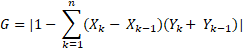
The calculation of the Gini coefficient can be performed in a number of ways. For simplicity and practicality, The DHS Program calculates the Gini coefficient with the Brown Formula shown below:
G: Gini coefficient
Xk: cumulative proportion of the population variable, for k = 1,...,n, with X0 = 0, Xn = 1
Yk: cumulative proportion of the wealth variable, for k = 1,...,n, with Y0 = 0, Yn = 1
and n = 100 in the DHS implementation.
To implement this, the following steps are used for each background characteristic:
1) Calculate the minimum (min) and maximum (max) wealth index score for the characteristic (national, urban/rural, or region). Note that min and max can be negative for specific characteristics, but at the national level min should be negative and max should be positive.
2) Calculate the wealth group k for each household as
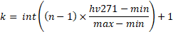
where n=100. This will result in groups 1 to 100.
3) Tally the population for each group k

where sample weight = hv005/1000000 and number of de jure household members = hv012.
4) Tally the relative wealth score for each group k by adding the weighted difference in wealth index score and minimum wealth index score for the background characteristics

5) Calculate cumulative population groups by accumulating the populations in each group k where k = 1 to 100 and cum.pop0 = 0

6) Calculate cumulative wealth groups by accumulating the relative wealth in each group k where k = 1 to 100 and cum.wealth0 = 0

7) Convert cumulative populations into cumulative proportions of population in each group k where k = 1 to 100

cum.pop100 is the total population for the characteristic as calculated in step 5, and prop.pop100 will thus be 1, and prop.pop0 = 0.
8) Convert cumulative wealth into cumulative proportions of wealth in each group k where k = 1 to 100

cum.wealth100 is the total relative wealth for the characteristic as calculated in step 6, and prop.wealth100 will thus be 1, and prop.wealth0 = 0.
9) Apply the formula given above to calculate the Gini coefficient (G), where k = 1 to 100.

There are no missing data for the wealth index factor score.
In addition to standard background characteristics, most of the results in the survey reports are shown by wealth quintiles, an indicator of the economic status of households. Although surveys under The DHS Program do not collect data on consumption or income, they do collect detailed information on dwelling and household characteristics and access to a variety of consumer goods and services, and assets, which together are used as a measure of economic status. The wealth index is a measure that has been used in many DHS and other country-level surveys to indicate inequalities in household characteristics, in the use of health and other services, and in health outcomes. The resulting wealth index is an indicator of the level of wealth that is consistent with expenditure and income measures. The wealth index is constructed using household asset data via principal components analysis.
In its current form, which takes better account of urban-rural differences in the scores and indicators of wealth, the wealth index is created in three steps. In the first step, a subset of indicators common to both urban and rural areas is used to create wealth scores for households in both areas. Categorical variables to be used are transformed into separate dichotomous (0-1) indicators, as are groupings of certain discrete variables such as numbers of different types of animals. These variables and those that are continuous are then analyzed using principal components analysis to produce a common factor score for each household. In a second step, separate factor scores are produced for households in urban and in rural areas using area-specific indicators. The third step combines the separate area-specific factor scores to produce a nationally applicable combined wealth index by adjusting the area-specific score through regression on the common factor scores. This three-step procedure permits greater adaptability of the wealth index in both urban and rural areas. The resulting combined wealth index has a mean of zero and a standard deviation of one, and once it is obtained, national-level wealth quintiles are obtained by assigning the household score to each de jure household member, ranking each person in the population by their score and then dividing the ranking into five equal parts, from quintile one (lowest-poorest) to quintile five (highest-wealthiest), each having approximately 20% of the population.
DHS-8 standard Table 2.6 shows the distribution across the five wealth quintiles of the population of urban and rural areas and in each region. These distributions indicate the degree to which wealth is evenly (or unevenly) distributed by geographic areas. The distribution of households by quintiles is not exactly 20 percent due to the fact that members of the households, not households, were divided into quintiles.
Also included in DHS-8 standard Table 2.6 is the Gini coefficient, which indicates the level of concentration of wealth, 0 being an equal distribution and 1 a totally unequal distribution. In other words, if every person in the country owned the same amount of wealth, the Gini coefficient would be 0. If one person in the country owned all of the wealth, then the Gini coefficient would be 1. In a country with a Gini coefficient of 0.2, wealth is fairly evenly distributed across the population. On the other hand, in a country with a Gini coefficient of 0.8, the top 10 percent of wealthiest people own much more wealth than the lowest 10 percent. A Gini coefficient that increases over time in a country indicates that wealth is becoming more concentrated, and disparities between the richest and poorest are increasing.
The Gini coefficient is calculated as a ratio of the areas on the Lorenz curve diagram (see figure below). If the area between the line of perfect equality and Lorenz curve is A, and the area underneath the Lorenz curve is B, then the Gini coefficient is A/(A+B). This ratio is expressed as a percentage or as the numerical equivalent of that percentage, which is always a number between 0 and 1. As wealth becomes more concentrated, the Lorenz curve moves down and to the right, area A increases as a proportion of A+B, and the Gini coefficient gets higher (closer to 1).
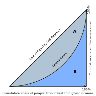
Source: https://en.wikipedia.org/wiki/Gini_coefficient
Because of its nature, smaller areas are more likely to have lower values of the Gini coefficient because they are more likely to be homogeneous than larger areas. Thus, the value of the coefficient in each region is often lower than the value of the nation as a whole.
The method of calculating the wealth quintiles has gone through several iterations. Initially the national wealth index score was calculated directly using a single principal components analysis (Rutstein and Johnson, 2004). In 2008 the calculation method was changed to produce separate urban and rural wealth scores and then use a regression equation to map these to a combined national wealth index score (Rutstein, 2008).
Rutstein, S.O. and K. Johnson. 2004. The DHS wealth index. DHS Comparative Reports No. 6. Calverton, Maryland, USA: ORC Macro. https://dhsprogram.com/publications/publication-cr6-comparative-reports.cfm
Rutstein, S.O. 2008. The DHS wealth index: Approaches for rural and urban areas. DHS Working Papers No. 60. Calverton, Maryland, USA: Macro International. https://dhsprogram.com/publications/publication-wp60-working-papers.cfm
Rutstein, S. O. and S. Staveteig. 2014. Making the Demographic and Health Surveys Wealth Index comparable. DHS Methodological Reports No. 9. Rockville, Maryland, USA: ICF International. https://dhsprogram.com/publications/publication-mr9-methodological-reports.cfm
DHS-8 Tabulation plan: Table 2.6
API Indicator IDs:
HC_WIXQ_P_LOW, HC_WIXQ_P_2ND, HC_WIXQ_P_MID, HC_WIXQ_P_4TH, HC_WIXQ_P_HGH, HC_WIXQ_P_GNI